How far can a signal travel through a deep neural network?
August 2026
Every input to a deep neural network passes through many layers. When the weights are random, as they are at initialisation, one of two things happens along the way: the input's structure fades until all inputs look alike (order), or small differences between inputs grow until similar inputs look unrelated (chaos).
Which one happens is set by two numbers: the weight scale σw, how spread out the random weights are, and the bias scale σb. On the boundary between order and chaos a signal survives through any number of layers, which is where very deep networks can still be trained.
This note replicates Poole et al. (2016), who locate that boundary with mean-field theory, for networks with tanh activations. The four exhibits below run the theory and small simulated networks live in your browser; figures from the research runs are in the appendix.
AT A GLANCE
QuestionHow many layers can a signal survive?How many layers can a signal survive?
NetworkRandom weights, tanh activationsRandom weights, tanh activations
SettingsWeight scale σw, bias scale σbWeight scale σw, bias scale σb
MethodMean-field theory, checked by simulationMean-field theory, checked by simulation
Key resultThe boundary between order and chaosThe boundary between order and chaos
ReplicatesPoole et al. (2016)Poole et al. (2016)
AdvisorBilin ZhuangBilin Zhuang
PeriodOctober 2025 – presentOctober 2025 – present
Exhibit A shows the effect directly. It takes a circle of inputs and pushes it through three random networks that differ only in their weight scale. With small weights the circle stays a smooth loop and shrinks (order); with large weights it crumples into a random walk (chaos).
EXHIBIT A: A CIRCLE THROUGH DEPTH
3 TANH NETWORKS, WIDTH 200, σb 0.3SIMULATED IN YOUR BROWSER
LAYER: 00 OF 30NETWORK: #0001
σw 1.2σw 2.5σw 4.0
χ1 0.87 ORDEREDχ1 1.59 CHAOTICχ1 2.37 CHAOTIC
LENGTH ×1.00LENGTH ×1.00LENGTH ×1.00
REPLAY SPEED
EACH PANEL: THE CIRCLE ON ITS TWO WIDEST DIRECTIONS (PCA), RESCALED TO FIT. LENGTH: CURVE LENGTH OVER LAYER 0. A NEW NETWORK IS DRAWN AFTER LAYER 30.
01. THE IDEA
Borrow the dictionary of phase transitions and point it at a network. Depth plays the role of distance, and the correlation length becomes the number of layers a pattern can survive. The edge of chaos is the knife-edge where that survival depth diverges: a network sitting there passes a signal through arbitrarily many layers without fading it or scrambling it.
PhysicsNetwork
Distance, or timeDepth, in layersDepth, in layers
Two-point correlatorActivation covarianceActivation covariance
Correlation length ξSurvival depth: layers a pattern lastsSurvival depth: layers a pattern lasts
Critical pointEdge of chaosEdge of chaos
02. TWO NUMBERS PER LAYER
At large width, each pre-activation is a sum of many independent random terms, so it is Gaussian. A whole layer then reduces to two numbers: the variance q of its pre-activations, and the correlation c between the images of two inputs. A layer with weight scale σw, bias scale σb and width N maps both forward.
hl = Wl tanh(hl−1) + bl, Wij ~ N(0, σw2/N), bi ~ N(0, σb2)
03. SIGNAL LENGTH
The first number is the variance. Its map from one layer to the next has a single stable fixed point q*, and both theory and simulation reach it within a handful of layers. The weight scale σw sets where it sits. Dz below is the standard Gaussian measure.
ql = σw2 ∫ Dz tanh2(√ql−1 z) + σb2
EXHIBIT B: THE LENGTH MAP
q OUT VS. q IN, σb 0.3LINES: THEORY. RINGS: ONE NETWORK, WIDTH 300
σw FIXED POINT q* 4.08
LAYER: 00 OF 10RUN: #0001
THEORY: 0.35 · 3.15 · 6.65SIMULATED: 0.35 · 3.15 · 6.65
REPLAY SPEED
DASHED: q OUT = q IN, AND q* ON THE RIGHT. EACH STAIR IS ONE LAYER, FROM THREE STARTING VARIANCES. OPEN CIRCLE: THE FIXED POINT.
04. ORDER VS. CHAOS
The second number is the correlation between two inputs as they descend. Below the critical weight scale, every pair is pulled together until c = 1, and the network forgets which input it saw: order. Above it, nearby inputs are pushed apart until they settle at a fixed point c* below 1: chaos. The crossover is sharp.
cl = [σw2 ∫ Dz1 Dz2 tanh(u1) tanh(u2) + σb2] / q*
u1 = √q* z1, u2 = √q* (cl−1 z1 + √(1 − (cl−1)2) z2)
EXHIBIT C: THE CORRELATION MAP
TWO INPUTS AT A TIME, σb 0.3LINES: THEORY. RINGS: ONE NETWORK, WIDTH 400
σw χ1 1.59 CHAOTIC, c* 0.12
LAYER: 00 OF 25RUN: #0001
THEORY: 0.10 · 0.50 · 0.90SIMULATED: 0.10 · 0.50 · 0.90
REPLAY SPEED
DASHED: c OUT = c IN, AND c* ON THE RIGHT. ORDERED NETWORKS PULL EVERY PAIR TO c = 1; CHAOTIC ONES SETTLE BELOW IT.
05. THE PHASE BOUNDARY
Whether c = 1 is stable comes down to one slope, χ1: how much a small perturbation grows from one layer to the next. Below 1, perturbations die out and the network is ordered; above 1, they grow and it is chaotic. Setting χ1 = 1 traces the boundary across the plane of bias and weight scales.
χ1 = σw2 ∫ Dz [tanh′(√q* z)]2
Near that line the survival depth ξ = −1 / ln χc grows without bound, where χc is the slope of the correlation map at its fixed point (equal to χ1 on the ordered side). A network initialised on the line can carry a signal through any depth, which is where very deep networks remain trainable [2].
EXHIBIT D: THE PHASE DIAGRAM
TANH NETWORKS: σb 0–4 ACROSS, σw 1–5 UPMEAN-FIELD THEORY
PRINTED: 00 OF 32 ROWSCLICK OR USE ARROW KEYS TO PROBE
PROBE: σw 2.50, σb 0.30q* 4.08
χ1 1.585: CHAOTICSURVIVAL DEPTH 5.1 LAYERS
● CHAOTIC, χ1> 1● ORDERED, χ1< 1- - - χ1 = 1○ EXHIBIT A'S NETWORKS
06. WHAT'S NEXT: MODE-SELECTIVE CRITICALITY
The clean theory treats every neuron alike. Give the network a symmetry instead, such as neurons on a ring whose connections depend only on the distance between them, and the same dictionary extends: the activations split into Fourier modes, and each mode gets its own critical point. The working hypothesis is mode-selective criticality: broad patterns survive to any depth while fine detail dies out, and the network's wiring alone decides which.
A perfectly symmetric ring keeps its modes clean and independent, like a crystal. Real networks break the symmetry and the modes blur together, like a liquid. That is where the closed-form theory stops and the next step begins: a sparse autoencoder, used the way a physicist uses a scattering experiment, to read the hidden modes back out.
PhysicsNetwork
Normal modesFourier modes of the activationsFourier modes of the activations
CrystalSymmetric ringSymmetric ring
LiquidBroken symmetryBroken symmetry
Scattering experimentSparse autoencoderSparse autoencoder
NOTES
What does mean-field mean here?
At large width each pre-activation sums many independent random terms, so it is Gaussian, and a layer is described by two numbers: q and c.
Are the exhibits the research runs?
No. They run the same equations with smaller networks, in your browser. Figures from the research runs are in the appendix.
Where is the code?
REFERENCES
[1]B. Poole, S. Lahiri, M. Raghu, J. Sohl-Dickstein and S. Ganguli. Exponential expressivity in deep neural networks through transient chaos. NeurIPS, 2016.
[2]S. S. Schoenholz, J. Gilmer, S. Ganguli and J. Sohl-Dickstein. Deep information propagation. ICLR, 2017.
[3]H. Sompolinsky, A. Crisanti and H.-J. Sommers. Chaos in random neural networks. Physical Review Letters 61, 259, 1988.
APPENDIX: FIGURES FROM THE RESEARCH RUNS
These come from the research code rather than the browser: the experiments behind Exhibits A to C, with simulations at width 1,000.
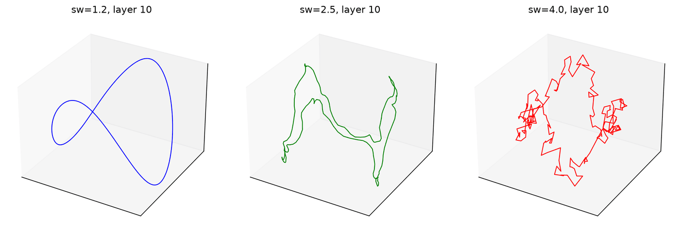
FIGURE A1: A CIRCLE AT LAYER 10σw 1.2 · 2.5 · 4.0
The same circle of inputs after ten layers. At σw = 1.2 it is still a smooth loop, at 2.5 it wrinkles, and at 4.0 it is a random walk.
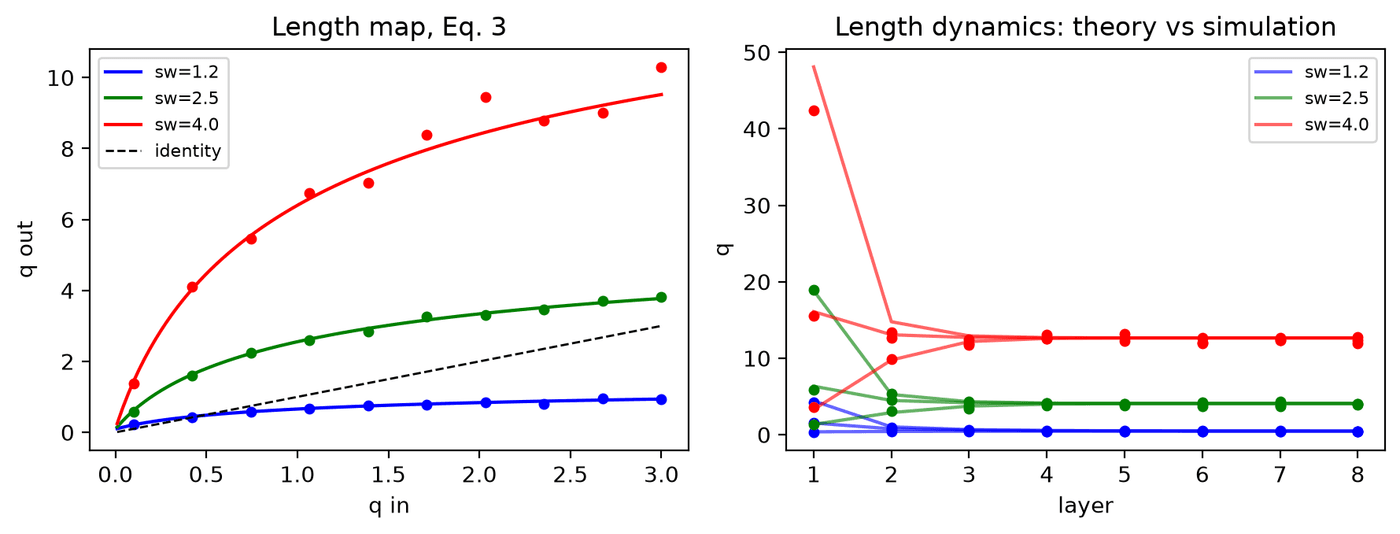
FIGURE A2: LENGTH MAP AND DYNAMICSTHEORY VS. SIMULATION
Left: the length map at three weight scales, against the identity line. Right: the variance against depth. Simulation points sit on the mean-field curves, and every start reaches its fixed point within a few layers.
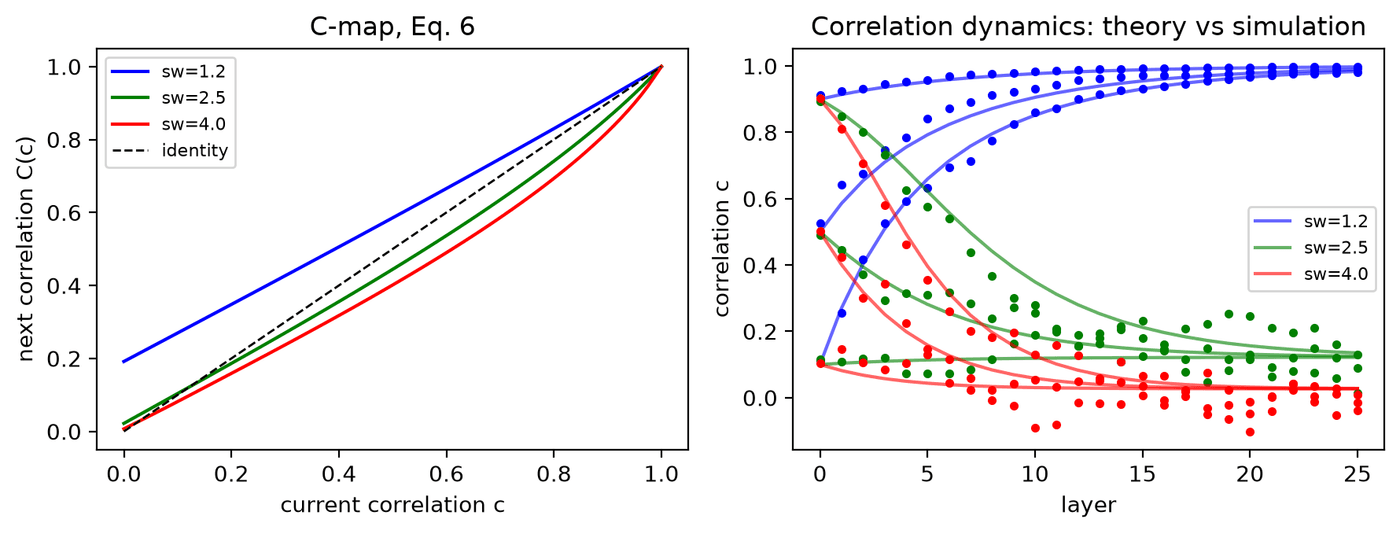
FIGURE A3: CORRELATION MAP AND DYNAMICSTHEORY VS. SIMULATION
Left: the correlation map. Right: the correlation against depth from three starting values. At σw = 1.2 every pair climbs to c = 1; at 2.5 and 4.0 the pairs settle at a fixed point below 1.
*** END OF NOTE ***